Elijah Cole
FMs and Perturbation Prediction: Performance Limits
This post discusses results from Foundation Models Improve Perturbation Response Prediction - check out the paper for full details. All opinions are my own.
TLDR: We built a “progress bar” for perturbation prediction tasks. Some are basically saturated; others have lots of headroom left.
Introduction
There is a lot of work on perturbation prediction, but it’s often unclear how much progress is really being made.
We can solve at least part of this problem. Given a specific problem formulation, we estimate two quantities: the best achievable performance (BAP) and the worst acceptable performance (WAP). The gap between these two values - the BAP-WAP gap, if you’re feeling whimsical - defines the range of “interesting” performance levels. For any given model, we can then compute the percentage of the BAP-WAP gap it closes. This functions like a progress bar for the task, allowing us to say something definitive about whether a particular problem is solved or has substantial remaining headroom.
For example, here’s what those results look like for the log fold change regression task on each cell line in the Essential dataset:
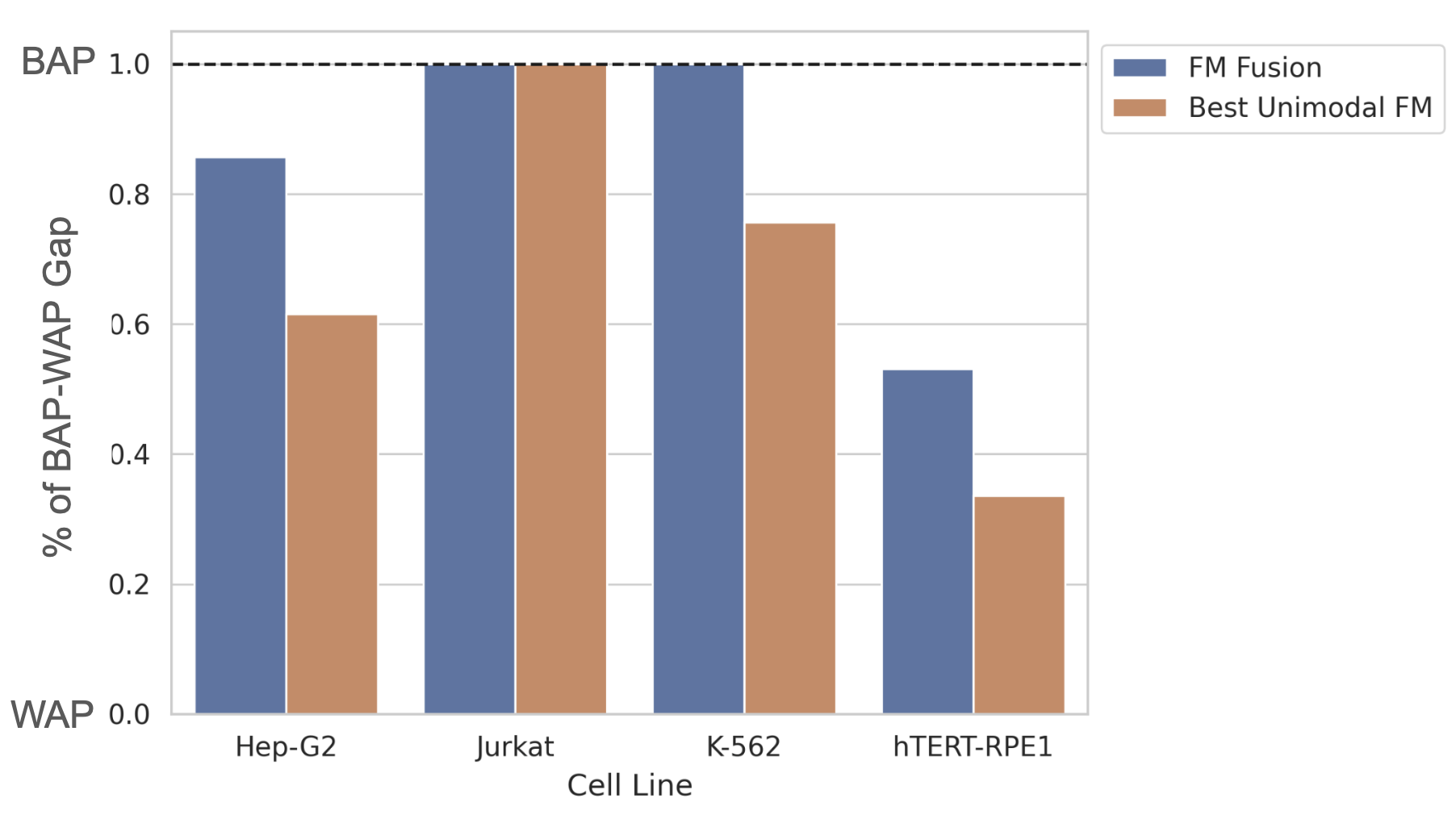
The orange bars represent the best unimodal foundation model (FM) embeddings and the blue bars represent a fusion model we propose in the paper. This figure shows that the Jurkat task is basically solved, while there’s plenty of headroom left on hTERT-RPE1.
Setup
Our work focuses on the problem of predicting the effect of unseen perturbations in a known cell line context.
We take an embedding-centric approach to this problem, evaluating models of the form
average_treatment_effect = f(pert_embedding)
where f is a simple predictor (e.g. kNN, lasso) and pert_embedding is some representation of the perturbation whose effect we want to predict. The protocol for training f is held constant, so the only variable is the perturbation embedding method. For fairness, we project all embeddings to the same dimension common_dim.
Best Achievable Performance (BAP)
By comparing a model to the best achievable performance, we can see how much room for improvement remains. Let’s suppose we have a collection of “cheater” methods that have unreasonable advantages. Then (assuming that higher is better) we can estimate the BAP by taking the minimum performance (or maximum error) over all cheater methods:
best_achievable_performance = min({cheat_method_i_performance})
Each cheater method represents an upper bound on the achievable performance, so we take the minimum to get the tightest bound on the BAP.
Our work considers two cheater methods.
Cheater Method 1: Idealized Baseline
If we restrict our attention to linear models, then we can use PCA to construct the optimal embeddings of dimension common_dim for predicting the labels (both train and test). In this paper, we call this method the idealized baseline:
Y = concat([Y_train, Y_test]) ... # (num_perturbations_train + num_perturbations_test) x num_genes
perturbation_embeddings = get_principal_components(Y.T, common_dim) # (num_perturbations_train + num_perturbations_test) x common_dim
This is not actually a hard ceiling, since nonlinear models can in principle produce better embeddings. Reasonable people could disagree about whether to include this in the BAP estimate. We expect this to be a very optimistic performance estimate, so we included it.
Cheater Method 2: Experimental Error (Test Data Bootstrapping)
Suppose we repeat the same perturbation experiment several times with different labs, reagent shipments, and personnel. We will observe some variability in the observed treatment effect y_obs. We can write this as y_obs = y_true + err_exp where err_exp is a random variable that represents the experimental error. (Note that the previous discussion was in terms of “higher is better” metrics - keep in mind that higher error = lower performance.)
We only have access to y_obs when training models; we never see y_true. A perfect model that predicts y_pred = y_true would satisfy E[||y_pred - y_obs||^2] = E[||err_exp||^2].
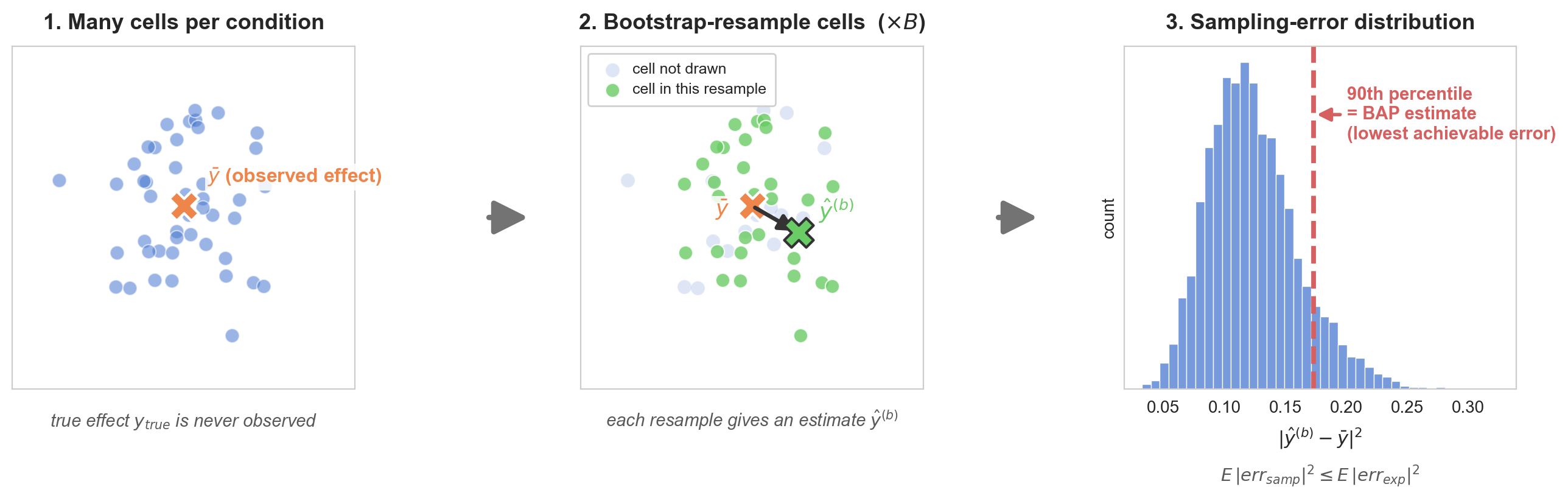
Our paper introduces a bootstrapping-based procedure for bounding E[||err_exp||^2]. We’ll leave full details to the paper and code, but the short version is:
- The perturbation datasets we consider consist of scRNA-seq, which gives us many replicates for the same conditions.
- Because our treatment effects are based on aggregating measurements from many cells, we can bootstrap to estimate the distribution of the error due to cell sampling,
err_samp. - Since
err_exp = err_samp + err_lots_of_other_stuff, we can boundE[||err_exp||^2] >= E[||err_samp||^2](assuming the error sources are independent). - Finally, we take the 90th percentile of the distribution of
E[||err_samp||^2]as an estimate of the best achievable performance / lowest achievable error.- Interpretation: Suppose a model’s error sits at the BAP estimate we’ve just described. Because this is the 90th percentile of the distribution of
E[||err_samp||^2], that means the model’s error is lower than the cell sampling noise 10% of the time.
- Interpretation: Suppose a model’s error sits at the BAP estimate we’ve just described. Because this is the 90th percentile of the distribution of
Worst Acceptable Performance (WAP)
On the low end, the worst possible performance is not very interesting. For a given metric (e.g. accuracy) it’s usually just some fixed value (e.g. zero in the case of accuracy).
What we care about instead is the worst acceptable performance. For a given problem, the worst acceptable performance is typically taken to be the maximum performance (assuming that higher is better) over some set of “null” methods that any sensible model should beat:
worst_acceptable_performance = max({null_method_i_performance})
Each null method represents a lower bound on the acceptable performance, so we take the maximum to get the tightest bound on the WAP.
Our work includes four of these null methods.
Null Method 1: Train Mean
Predict the effect of perturbation p in cell line c as the average of all training perturbations for c. This prediction ignores p.
Null Method 2: No Change
Predict the effect of perturbation p in cell line c as the control expression for c. This is equivalent to predicting that p has no effect in c.
Null Method 3: Random Embeddings
Represent each perturbation p with a random vector, e.g. a vector with entries that are IID draws from a standard normal distribution. Obviously these embeddings carry no information about the relationship between different perturbations. A supervised model trained on these embeddings cannot generally do any better than predicting the train mean.
Null Method 4: PCA-Derived Embeddings
For the problem of genetic perturbation prediction, perturbations are synonymous with genes. We can therefore come up with some simple gene embeddings using PCA:
Y_train = ... # num_perturbations x num_genes
pcs = get_principal_components(Y_train, num_components=common_dim) # num_genes x common_dim
To embed a given gene, we use the corresponding row of pcs. FM embeddings must beat PCA-derived embeddings to stand a chance of being worth the compute - see our prior blog post for more on that.
(This approach is not applicable for chemical perturbation modeling.)
Concluding Thoughts
Quantitative results are much more interesting if we can contextualize them with upper and lower limits. We can see whether we’re really advancing past naive baselines, and we can see whether the problem still has enough headroom to be interesting.
The idea is general, but the specific upper and lower bound methods will vary depending on how the problem is formulated. For instance, our bootstrapping method relies on the fact that we’re predicting average treatment effects derived from scRNA-seq data. It wouldn’t work if you just had one bulk measurement for each condition.
Key Takeaway: If we can estimate upper and lower bounds on performance, we can create a “progress bar” for each perturbation prediction task.